Language Models are models that are trained to predict the next word, given a set of words that are already uttered or written. e.g. Consider the sentence: “Don’t eat that because it looks…“
The next word following this will most likely be “disgusting”, or “bad”, but will probably not be “table” or “chair”. Language Models are models that assign probabilities to sequences of words to be able to predict the next word given a sequence of words.
The probability of a word $w$ given some history $h$ is $p(w|h)$.
N-Grams
The probability of a word $w$ given the history $h$ is defined as:
\[p(w|h)\]as $h$ is several tokens long, we can rephrase it as the probability of the ${n+1}^{th}$ word $w_{n+1}$ depends on the words $w_1, w_2 \cdots w_n$.
\[p(w_{n+1}|w_1, w_2, w_3 \cdots w_n)\]One way to answer this is using relative frequency counts. i.e. count the number of times we see $w_1, w_2, w_3 \cdots w_n$ and the number of times we see $w_1, w_2, w_3 \ldots w_n$ followed by $w_{n+1}$.
Relative frequency is defined as the ratio of an observed sequence to the observed sequence followed by a suffix. Using the concept of relative frequency we can get:
\[P(w_{n+1}|w_1 w_2 w_3 \ldots w_n) = \frac{C(w_1 w_2 w_3 \cdots w_n w_{n+1})}{C(w_1 w_2 w_3 \ldots w_n)}\]Where $C(x_1, x_2)$ is the count or the number of times we see a pattern of token $x_1$ followed by $x_2$.
This approach of getting probabilities from counts works well in many cases, but if we wanted to know the joint probability of an entire sequence of words $p(w_1, w_2, w_3 \ldots w_n)$, we would have to compute - out of all the possible combinations of size $n$ how many are this exact sequence $w_1, w_2, w_3 \ldots w_n$. It fails when the size of the sequence is very long.
Even the entire web isn’t big enough to compute such probabilities, because there are not enough examples for every word combination even on the world wide web). For this reason, we will have to introduce clever ways of computing probability.
Let’s decompose this joint probability into a conditional probabilities using the chain rule of probability.
Chain Rule of Probability helps us decompose a joint probability into a conditional probability of a word given previous words. Joint Probability of $n$ words is the probability of $n$ words occurring together. Using the chain rule, we can break down Equation the joint probability of a sequence of tokens into conditional probabilities. Here is how we do it:
\[\begin{eqnarray} P(w_1 w_2 w_3 \cdots w_n w_{n+1}) &=& P(w_1) P(w_2|w_1) P(w_3|w_1 w_2) \ldots P(w_n|w_1\ldots w_{n-1}) \nonumber \\ &=& \prod_{k=1}^{n+1} P(w_k|w_1 \ldots w_k) \end{eqnarray}\]The chain rule still has the constraint of needing the probability of a long sequence of previous words. One idea is to approximate this using the Markov Assumption.
Markov Assumption says that the probability of a word only depends on the previous word and not the entire sequence of tokens preceding it. According to this assumption, we can predict a word without looking too much into the previous history of words. So, instead of working with the exact probabilities of a long sequence of preceding words, we can use a small window of preceding words. This is where we introduce a bigram model (that uses the preceding word only) a trigram model (that uses the preceding two words) to predict the probability of a sequence of tokens.
Using the bigram model we can simplify the probability of a sequence of tokens to the following:
\[P(w_1, w_2, w_3 \cdots w_n, w_{n+1}) = \prod_{k=1}^n P(w_k|w_{k-1})\]Similarly using the trigram model we can simplify the probability of a sequence of tokens to the following:
\[P(w_1, w_2, w_3 \cdots w_n, w_{n+1}) = \prod_{k=1}^n P(w_k|w_{k-1} w_{k-2})\]Now that we have simplified the RHS, we need to compute the probabilities.
Maximum Likelihood Estimation (MLE) is an intuitive way of measuring the parameters of an N-gram model, by computing the counts of words or tokens that exist together, normalized by the total counts so that the output is a probability that is between 0 and 1. Relative frequency is one way of measuring the MLE. Relative frequency can be computed using equation (7) below and Figure (1) explains the equation:
\[P(w_n|w_{n-1}) = \frac{C(w_{n-1}w_n)}{\sum_w C(w_{n-1}w)}\]
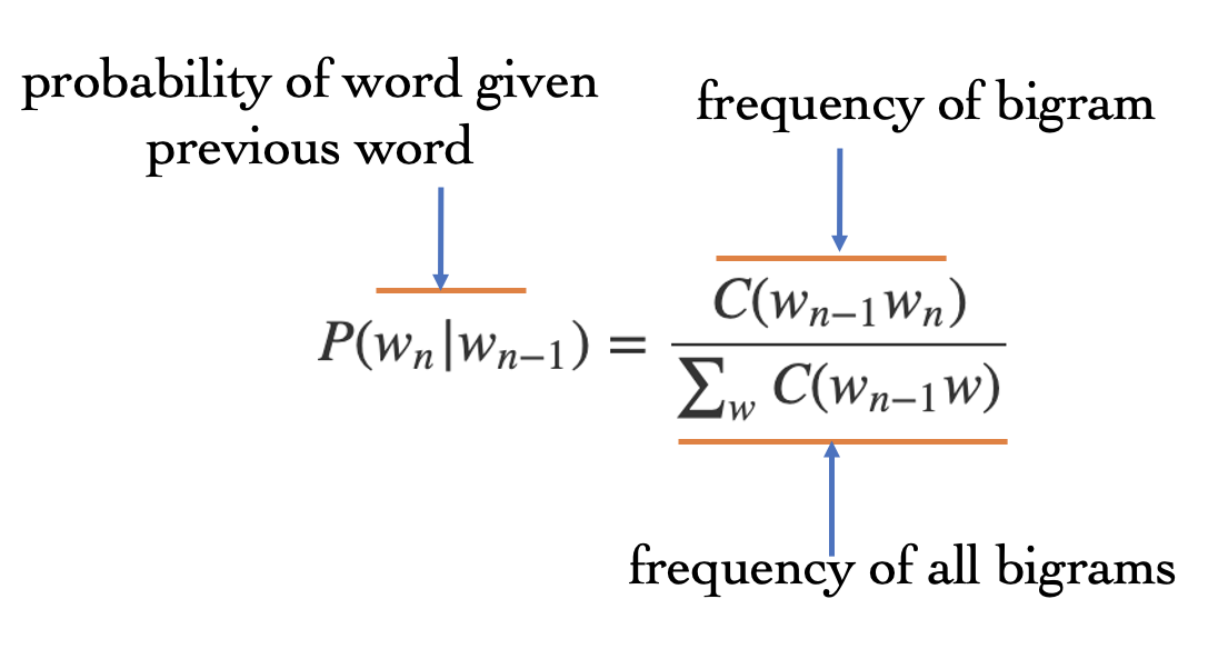
Fig 1: Relative Frequency Explained
Working Example
Let’s build a small language model using bigrams, and use our model to predict the probability of a new sentence. For our toy example, consider a tiny corpus of the following sentences:
<s> I am Sam <\s>
<s> Sam I am <\s>
<s> I do not like that Sam I am <\s>
Here <s> represents the start of a sentence and <\s> represents the end of the sentence.
This corpus has the following lexicon or unique words:
| token | frequency |
| I | 4 |
| am | 3 |
| Sam | 3 |
| do | 1 |
| not | 1 |
| like | 1 |
| that | 1 |
Computing the conditional probabilities
\[P(I|<s>) = \frac{2}{4}\] \[P(Sam|<s>) = \frac{1}{3}\] \[P(am|I) = \frac{3}{4}\]We can continue computing probabilities for all different possibilities of bigrams, then for any new sentence such as the following:
I like Sam
We can compute the join probability of the tokens of this sentence from the conditional probability of the bigrams $P(like|I)$ and $P(Sam|like)$.
Practical Issues
- Always use Log probabilities. Multiplication in linear space is addition in log space, and we will avoid numerical underflow
- It is typical to use trigrams instead of bigrams (although we illustrated bigrams in the example above)
- There are often unknown words in the sentence we want to predict the probability of, and we need to handle that.
- We often won’t find instances of joint probability in our corpus, and we need to account for that. E.g. in the above example we do not have an instance of ‘sam like’, and so the conditional probability of $P(Sam|like)$ will be $0$.
Problems with language Models
Language Models face the issue of sparsity - which means that the training corpus is limited and some perfectly acceptable English word sequences are bound to be missing from it. This means that it is possible to have several n-grams with a probability of $0$, but should actually have a non-zero probability.
Another issue with language models is that the vocabulary the the language model is trained on might not have seen words from the test dataset - introducing the issue of unknown words or out of vocabulary words(OOV). One way to deal with OOV words is to replace all words with a frequency below a certain threshold by ‘UNK’. Other ways to deal with this is to use smoothing and discounting techniques.
Smoothing
There will always be unknown words in the test dataset that the language model will have to work with that sparsity. To keep the language model from assigning zero probabilities to unseen events, we will shave off some probability mass from some more frequent events and give it to the events that we have never seen. This process is called smoothing or discounting.
A few types of smoothing are:
- add-1 smoothing (or Laplace smoothing)
- add-k smoothing
- backoff and interpolation
- stupid backoff
- Kneser ney smoothing
Laplace Smoothing
Laplace smoothing involves adding $1$ to all of the bigram (or n-gram) counts before we normalize them into probabilities.
\[P(w_i) = \frac{c_i}{N}\]If we add $1$ to each probability, and there are $V$ words in the vocabulary, we will need to add $V$ to the denominator as we add $1$ to each numerator.
\[P_{laplace}(w_i) = \frac{c_i}{N+V} \label{laplace}\]In equation \ref{laplace}, $w_i$ is the $i^{th}$ word, $N$ is a normalizer (total number of words) and $V$ is the vocabulary size.
But instead of adding to the numerator and denominator, a better way to is change the numerator only, and show how it affects smoothing by describing an adjusted count $c^*$.
\[c_i^* = (c_i + 1) \frac{N}{N+V}\]Now we can convert each adjusted count into a probability by dividing it by $N$ (the total number of tokens)
Although Laplace smoothing isn’t the best type of smoothing as it gives away a lot of probability mass to infrequent terms, it is still used and is practical for classification.
** Question: How can you use Language Models for classification? **
\[P(w_n|w_{n-1}) = \frac{C(w_{n-1} w_n)}{C(w_{n-1})}\]Using Laplace Smoothing, this becomes:
\[p^*_{Laplace}(w_n|w_{n-1}) = \frac{C(w_{n-1} w_n) + 1}{\sum_w C(w_{n-1}w) + V}\]Add-k smoothing
Add-K smoothing is an alternative to add $1$ smoothing, where we move a bit less of the probability mass from the seen events to the unseen events.
\[p^*_{add-k}(w_n|w_{n-1}) = \frac{C(w_{n-1} w_n) + k}{\sum_w C(w_{n-1}w) + kV}\]Add-K requires us to have a method for choosing our k (0.5? 0.1? 0.05?) e.g. one can optimize over a dev set or some other data source.
Backoff and Interpolation
Backoff is an approach for smoothing using which we only backoff to a lower order n-gram when we have zero evidence for a higher level n-gram.
So, we use a trigram if the evidence is sufficient, but if such a trigram does not exist, we backoff to a bigram, and if the bigram does not exist, we backoff to a unigram.
Interpolation is an approach is using a mixture of probability estimates from all the n-gram estimators. For instance, if we are looking at trigrams, we would compute its probability by combining the trigram, bigram and unigram counts.
Interpolation for a trigram can be defined by the following formula:
\[\hat{p}(w_n|w_{n-2}w_{n-1}) = \lambda_1 p(w_n|w_{n-2}w_{n-1}) + \lambda_2 p(w_n|w_{n-1}) + \lambda_3 p(w_n)\]where $\sum_i \lambda_i = 1$
The values of $\lambda$ can be computed by optimizing over a heldout dataset. EM Algorithm (Expectation Maximization Algorithm) is an iterative learning algorithm that converges on locally optimal $\lambda$s
Evaluating Language Models
There are 2 ways to evaluate language models:
- intrinsic evaluation: Evaluation of the model as a measure of how much it improves the application that it is used in.
- extrinsic evaluation: Measure of the quality of the model independent of any application
Intrinsic Evaluation
For intrinsic evaluation of a language model we need to have:
- training dataset
- test dataset
- held out dataset
We use the language model to compute scores on the test dataset, and use the heldout and training dataset to optimize out language model.
Extrinsic Evaluation
To compute extrinsic evaluation of a language model, we compute the effect of a new language model on the final end to end product that it is integrated with. Good scores during intrinsic evaluation does not always mean better scores during extrinsic evaluation, which is why both the types of evaluation are important.
Perplexity
Perplexity is the measure of computation of the probabilities learned from the training dataset and applied on the test dataset. Perplexity is represented as $PP$ and is measured as the inverse probability of the test set, normalized by the number of words.
\[\begin{eqnarray} PP(w) &=& P(w_1 w_2 w_3 \ldots w_n)^{-\frac{1}{n}} \nonumber \\ &=& \sqrt[n]{\frac{1}{P(w_1 w_2 w_3 \ldots w_n)}} \nonumber \\ &=& \sqrt[n]{\frac{1}{\prod_{i=1}^nP(w_i|w_1 w_2 \ldots w_{i-1})}} \end{eqnarray}\]To compute perplexity of a bigram, we can simplify Equation (11) to the following:
\[PP(w) = \sqrt[n]{\frac{1}{\prod_{i=1}^nP(w_i|w_{i-1})}}\]Similarly, to compute perplexity of a bigram, we can simplify Equation (11) to the following:
\[PP(w) = \sqrt[n]{\frac{1}{\prod_{i=1}^nP(w_i|w_{i-1} w_{i-2})}}\]Minimizing perplexity is equivalent to maximizing the test set probability. If the perplexity is low, it means that the training data captures the probability of the test set really well.
Another way to think about perplexity is to think of it as the weighted average branching factor of the language. The branching factor of a language is the number of possible next words that can follow any word.
Intrinsic improvement in perplexity does not guarantee an extrinsic improvement in the performance of the language processing task.
N-Gram Efficiency considerations
When a language model uses large sets of n-grams, it is important to store the efficiently. Below are some ways to store LMs efficiently:
- Words: storing words in 64 bit hash representations, and the actual words are stored on disc as string
- Probabilities: 4-8 bits instead of 8 byte float
- n-grams: Stored in reverse tries
- Approximate language models can be created using techniques such as bloom filters
- n-grams can be shrunk by pruning i.e. only storing n-grams with counts greater than some threshold.
- Efficient Language Models such as KenLM
- Use sorted Arrays
- Efficiently combined probabilities and backoffs into a single value
- Use merge sorts to efficiently build probability tables in a minimal number of passes through a large corpus
References
- Chapter 3, Speech and Language Processing: An Introduction to Natural Language Processing, Computational Linguistics, and Speech Recognition by Daniel Jurafsky, James H. Martin
- Language Models, Wikipedia
- Lecture 2, Language Models, CS224n Stanford NLP
- NLP Lunch Tutorial: Smoothing, Bill MacCartney, Stanford NLP
- Relative Frequency, mathisfun.com