The Comprehensive Guide to Logistic Regression

In Natural Language Processing (NLP) Logistic Regression is the baseline supervised ML algorithm for classification. It also has a very close relationship with neural networks (If you are new to neural networks, start with Logistic Regression to understand the basics.)

Introduction

Logistic Regression is a discriminative classifier.

Discriminative models try to learn to distinguish what different classes of data look like.

Some examples of discriminative classifiers are Logistic Regression, Neural Networks, Conditional Random Fields, and Support Vector Machines.

Naive Bayes, is a generative classifier.

Generative models have the goal to understand what different classes of data look like.

Some examples of generative classifiers include Naive Bayes, Bayesian Networks, Markov Random Fields, and Hidden Markov Models. LDA (Latent Dirichlet Allocation is a generative statistical model for topic modeling.

Ng and Jordan, 2001 provide a great analysis of generative vs discriminative models.

Components of a Classification System

A Machine Learning system for classification has 4 components:

Feature Representation: For each input observation $x^{(i)}$, this will be a vector of features $[x_1, x_2, x_3, … , x_n]$
A Classification Function: This gets us the probability of the output, given an input. This is denoted by $P(y|x)$. Sigmoid and Softmax are tools for classification for Logistic Regression.
Objective Function for Learning: This is the function that we want to optimize, usually involving minimizing error on training examples. Cross Entropy Loss is the objective function for Logistic Regression.
Algorithm for Optimizing the Objective Function: We use the Stochastic Gradient Descent Algorithm for optimizing over our Objective Function.

Logistic Regression Phases

Logistic Regression has two phases:

Training Phase: We train the system (specifically the weights $w$ and bias $b$) using Stochastic Gradient Descent and Cross Entropy Loss
Test Phase: Given a text example $x$, we compute $p(y|x)$ and return the higher probability label.

Feature Representation

A single input observation $x$ can be represented by a vector of features $[x_1, x_2, x_3, \ldots , x_n]$. For Logistic Regression this is usually done by feature engineering which is the process of manually identifying which features are relevant to solve the problem, and convert the text features into real numbers.

Feature Interactions: Feature Interaction is the combination of different features to form a more complex feature.

Feature Templates: Feature Templates is when templates are used to automatically create features using abstract specification of features.

Representation Learning: Representation Learning is the process of learning features automatically in an unsupervised way from the input. In order to avoid the excessive human effort of feature design, recent NLP efforts are focused on representation learning

Classification using the Sigmoid Function

The result of Logistic Regression is:

\[z = (\sum_{i=1}^n w_i x_i) + b\]

Here, $w_i \cdot x_i$ is the dot product of vectors $x_i$ and $w_i$ and $z$ is a real number vector ranging from $-\infty$ to $+\infty$

Dot Product: The dot product of 2 vectors $a$ and $b$ is written as $a \cdot b$ and is the sum of the products of the corresponding elements of each vector.

$z$ is not a legal probability. To make it a probability, $z$ will pass through the, written as $\sigma(z)$

\[y = \sigma(z) = \frac{1}{(1+e^{-z})}\]

Image of Sigmoid Function
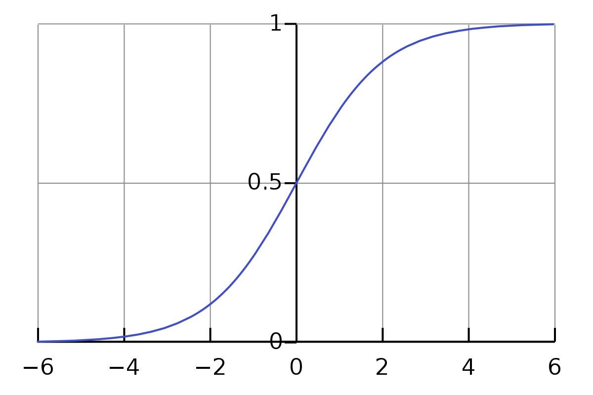
Fig 1: Sigmoid Function (Image Credit: Wikipedia)

Characteristics of Sigmoid Function

Sigmoid takes a real valued number and maps it to the range [0, 1] (which is perfect to get a probability)
Sigmoid tends to squash outlier values towards 0 or 1
Sigmoid is differentiable - which makes it handy for learning (A function is not differentiable if it has a undefined slope or a vertical slope)

For classification into two classes:

\[\begin{eqnarray} p(y=1) &=& \sigma(w \cdot x) + b \nonumber \\ &=& \frac{1}{1+e^{w.x + b}} \end{eqnarray}\] \[\begin{eqnarray} p(y=0) &=& 1 - \sigma(w \cdot x) + b \nonumber \\ &=& 1 - \frac{1}{1+e^{w.x + b}} \nonumber \\ &=&\frac{e^{w.x + b}}{1+e^{w.x + b}} \end{eqnarray}\]

Learning Process in Logistic Regression

Cost Function: Cross Entropy Loss

Cross Entropy Loss is a function that determines for an observation $x$, how close the output of the classifier $\hat{y}$ is to the correct output $y$. This $Loss$ is expressed as: $ L(\hat{y}, y) $

$ L(\hat{y}, y)$ is computed via a loss function that prefers the correct class labels of the training examples to be more likely. This is called conditional maximum likelihood estimation. We choose parameters $w$ and $b$ that maximize the probability of the true $y$ labels in the training data given the observations $x$.

Given a Bernoulli Distribution (a distribution that can only have 2 outcomes):

\[p(y|x) = \hat{y}^y (1-\hat{y})^{1-y}\]

Taking log on both sides:

\[\log{p(y|x)} = y\log{\hat{y}} + (1-y)\log{(1-\hat{y})}\]

Equation (6) is what we are trying to maximize. In order to turn this into a loss function (something that we need to minimize), we just flip the sign on Equation $(6)$. The result is Cross Entropy Loss $L_{CE}$.

\[\begin{eqnarray} L_{CE}(\hat{y}, y) &=& -\log{ p(y|x)} \nonumber \\ &=& -[y \log{\sigma(w \cdot x + b) + (1-y)\log(1-\sigma(w \cdot x + b))}] \end{eqnarray}\]

Equation (7) is known as the cross entropy loss. It is also the formula for the cross entropy between the true probability distribution $y$ and the estimated distribution $\hat{y}$.

Cross Entropy

Cross Entropy is the measure of the difference between two probability distributions for a given random variable.

Convex Optimization Problem

For logistic regression the loss function is convex, i.e. it has just one minimum. There is no local minima to get stuck in, so gradient descent will always find the minimum. The loss for multi-layer neural networks in non-convex, so it is possible to get stuck in local minima using neural networks.

Decision Boundary

Decision Boundary is the threshold above which $\hat{y} = 1$, and below which $\hat{y} = 0$. This means that the decision boundary decides which class a given instance belongs to, based on the final probability of the item and the value of the decision boundary.

\[\hat{y} = \left\{ \begin{array}{ll} 1 & \mbox{if $p(y=1|x)$ $\gt$ 0.5}\\ 0 & \mbox{otherwise} \end{array} \right.\]

Here 0.5 is the decision boundary, and it is the threshold that decides which class an item belongs to.

Gradient Descent

Gradient Descent finds the gradient of the loss function at the current point (by taking a differential of it), and then moves in the opposite direction of gradient.

Learning Rate

The magnitude of the amount to move in gradient descent is the slope $ \frac{d}{dw} \; f(x,w)$ weighted by the learning rate $\eta$.

\[w^{t+1} = w^{t} - \eta \; \frac{d}{dw} \; f(x; w)\]

Learning Rate: A parameter that needs to be adjusted:

If the learning rate is too high, each step towards learning becomes too large and it overshoots the minimum
If the learning rate is too low, each step is too small and it takes a long time to get to the minimum
Start $\eta$ at a higher value and slowly decrease it, so that it is a function of the iteration $k$ in training

Stochastic Gradient Descent

It is called Stochastic Gradient Descent because it chooses a single random example at a time. It moves weights so that it can improve the performance of that single instance.

Batch Training

When we use Batch Training, we compute the gradient over the entire dataset. It looks at all the examples for each iteration to decide the next step.

Mini-Batch Training

We train a group of $m$ examples (where $m$ is 512, or 1024 or similar) that is less than the size of the entire dataset. When $m = 1$ it becomes Stochastic Gradient Descent again. Mini-Batch Training is more efficient than Batch Training and more accurate than Stochastic Gradient Descent. Mini-Batch Gradient Descent is the average of the individual gradients.

Regularization

Regularization is used to avoid overfitting and to generalize well for the test data. If the model fits the training data too well, it will not be able to handle new cases presented in the test data.

A regularization term $R(\theta)$ is added to the objective function. i.e. the function that computes $\hat{\theta}$, where $\hat{\theta}$ is the next set of $w$ and $b$ parameters.

Once we add regularization, we can find $\hat{\theta}$ as:

\[\hat{\theta} = argmax_{\theta} \sum_{i=0}^m log(p(y^{(i)}\|x^{(i)})) - \alpha R(\theta)\]

Here we are maximizing the log probability instead of minimizing the loss (Equation (7)).

$R(\theta)$ is used to penalize large weights. The intuition behind this is that if the model matches the training data perfectly, but uses large weights, then it will be penalized more than the case where the model matches the training data a little less, but does so using small weights.

L2 Regularization

L2 Regularization is the euclidean distance of the vector squared from the origin.

$ R(\theta) = || \theta ||_2^2$ Is the notation of L2 Norm

$ R(\theta) = \sum_{j=1}^n \theta_j^2$ Is how we can compute L2 Norm

L2 regularization is easy to optimize because of it’s simple derivative. It prefers weight vectors in smaller weights.

L1 Regularization

L1 Regularization is the linear function named after L1 norm or Manhattan Distance, which is the sum of the absolute values of the weights.

$R(\theta) = || \theta ||_1$ is the notation of L1 norm

L1 Regularization is hard to differentiate as the derivative of $| \theta |$ is non continuous at 0. It prefers sparse solutions with larger weights.

Multinomial Logistic Regression

[Multinomial Logistic Regression]() is also known as Softmax Regression or Maxent Classifier. In Multinomial Logistic Regression the target variable $y$ ranges over more than two classes.

In order to support more than 2 classes, Multinomial Logistic Regression uses the softmax function instead of the sigmoid function.

For a vector $Z$ of dimensionality $k$ the softmax function is defined as:

\[Softmax(Z_i) = \frac{e^{z_i}}{\sum_{j=1}^k e^{z_j}}\]

In the above equation the denominator helps normalize the values into probabilities.

Like Sigmoid, Softmax has the property of squashing values towards 0 or 1
If one of the inputs is larger than the others, it will tend to push its probability towards 1, and suppress the probabilities of the smaller inputs.

Loss Function in Multinomial Logistic Regression

To compute the loss function in Multinomial Regression, we need to account for $k$ classes that a given item can belong to (instead of just 2 classes) $\begin{eqnarray} L_{CE}(\hat{y}, y) &=& - \sum_{k=1}^k 1 \{y=k\} log p(y=k|x) \nonumber \\ &=& - \sum_{k=1}^k 1 \{y=k\} log \frac{e^{w_k \cdot x + b}}{\sum_{j=1}^k e^{w_j \cdot x + b_j}} \end{eqnarray}$

In equation (11) $ 1{ }$ evaluates to 1 if the condition in the brackets is true, and $0$ otherwise.

Working Example of Logistic Regression

Consider a simple scenario where we are doing sentiment analysis of a dataset, and we have 2 classes: positive and negative (there is no neutral class in our hypothetical scenario). In this example we will be using the sigmoid function (because we have only 2 classes, and for simplicity we will not be using any regularization.

The following are the matrices representing the actual outcome $y$ and the features corresponding to it $x$.

$y = \begin{pmatrix}y\\1 \\ 0\end{pmatrix} \;\; x = \begin{pmatrix}x1 & x2 \\ 3 & 2\\ 1 & 3\end{pmatrix}$

In this example we have only 2 features $x_1$ and $x_2$. $x1$ is the number of positive words found in the sentence and $x2$ is the number of negative words found in the sentence. Also, $y=0$ represents negative (or bad sentiment), and $y=1$ represents positive (or good sentiment).

This stage is feature extraction and representation of our data.

The next state is to initialize out initial weights. For this example, we are setting $w_1 \; = \; w_2 \;= \; b \;= \; 0$.

($w_1$ is the weight of feature $x_1$ and $w_2$ is the weight of feature $x_2$), $\beta$ is our bias term.

$\eta \;= \; 0.1$

Each step in learning for logistic regression is represented by the following formula:

\[\theta^{t+1} = \theta^t - \eta \; \delta_\theta \; L(f(x^{(i)}, \theta), y^{(i)})\]

Here is a breakdown of each of the components of the formula.

Fig 2: Each step for Learning in Logistic Regression

Gradient Descent Step 1

Considering the first row, where $y=1$ finding the gradient for this example:

$ \delta_{wb} = \begin{pmatrix} \frac{\partial L_{CE}(w, b)}{\partial_{w_1}} \\ \frac{\partial L_{CE}(w, b)}{\partial_{w_1}} \\ \frac{\partial L_{CE}(w, b)}{\partial_{b}} \end{pmatrix}$

$ \delta_{wb} = \begin{pmatrix} (\sigma (w \cdot x + b) - y)) \; x_1 \\ (\sigma (w \cdot x + b) - y)) \; x_2 \\ \sigma (w \cdot x + b) - y \end{pmatrix}$

We know that initial $w, b = 0$. Substituting these values:

$ \delta_{wb} = \begin{pmatrix} (\sigma (0) - 1)) \; x_1 \\ (\sigma (0) - y)) \; x_2 \\ \sigma (0) - y \end{pmatrix}$

Given that $\sigma(0) = 0.5$ (See the sigmoid image above) and $x_1 = 3$ and $x_2 = 2$ for the first example in matrix $x$ (first row in matrix)

$ \delta_{wb} = \begin{pmatrix} (0.5 - 1) * 3 \\ (0.5 - 1) * 2 \\ 0.5 - 1 \end{pmatrix}$

$ \delta_{wb} = \begin{pmatrix} -1.5 \\ -1.0 \\ -0.5 \end{pmatrix}$

Now that we have the gradient, we can compute $\theta_1$ by moving in the opposite direction as the gradient.

$ \theta_{1} = \begin{pmatrix} w_1 \\ w_2 \\ b \end{pmatrix} - \eta \begin{pmatrix} -1.5 \\ -1.0 \\ -0.5 \end{pmatrix}$

Given that $w_1 = w_2 = b = 0$ and $\eta = 0.1$:

$ \theta_{1} = \begin{pmatrix} 0.15 \\ 0.1 \\ 0.05 \end{pmatrix}$

The weights after one step of gradient descent: $w_1 = 0.15$, $w_2 = 0.1$, $b = 0.05$.

Gradient Descent Step 2

This time we will consider row 2 of our matrix. The weights learned so far are : $w_1 = 0.15$, $w_2 = 0.1$, $b = 0.05$ The values from our matrix are $x_1 = 1$, $x_2=3$, $y=0$.

From Equation (9) computing the gradient:

$ \delta_{wb} = \begin{pmatrix} (\sigma (w \cdot x + b) - 0)) \; x_1 \\ (\sigma (w \cdot x + b) - 0)) \; x_2 \\ \sigma (w \cdot x + b) - y \end{pmatrix}$

$ \delta_{wb} = \begin{pmatrix} (\sigma (0.15 * 1 + 0.1 * 3 + 0.05) - 0) \; 1 \\ (\sigma (0.15 * 1 + 0.1 * 3 + 0.05) - 0) \; 3 \\ \sigma (0.15 * 1 + 0.1 * 3 + 0.05) - 0 \end{pmatrix}$

$ \delta_{wb} = \begin{pmatrix} (\sigma (0.15 + 0.3 + 0.05) - 0) \; 1 \\ (\sigma (0.15 + 0.3 + 0.05) - 0) \; 3 \\ \sigma (0.15 + 0.3 + 0.05) - 0 \end{pmatrix}$

Sigmoid of 0.5 is 0.622. (Compute your own sigmoid)

$ \delta_{wb} = \begin{pmatrix} (0.622 - 0) \; 1 \\ (0.622 - 0) \; 3 \\ 0.622 - 0 \end{pmatrix}$

$ \delta_{wb} = \begin{pmatrix} 0.378 \\ 1.134 \\ 0.378 \end{pmatrix}$

Now that we have the gradient, we can compute $\theta_2 $ by moving in the opposite direction as the gradient.

$ \theta_{2} = \begin{pmatrix} w_1 \\ w_2 \\ b \end{pmatrix} - \eta \begin{pmatrix} 0.378 \\ 1.134 \\ 0.378 \end{pmatrix}$

$ \theta_{2} = \begin{pmatrix} 0.15 \\ 0.1 \\ 0.05 \end{pmatrix} - 0.1 \begin{pmatrix} 0.378 \\ 1.134 \\ 0.378 \end{pmatrix}$

$ \theta_{2} = \begin{pmatrix} 0.15 - 0.0378 \\ 0.1 - 0.1134 \\ 0.05 - 0.0378 \end{pmatrix} $

$ \theta_{2} = \begin{pmatrix} 0.1122 \\ -0.0134 \\ 0.4622 \end{pmatrix} $

At the end of step 2, $w_1 = 0.1122$, $w_2 = -0.0134$ and $b = 0.04622$.

We can continue this process for $k$ number of steps and iterate through the examples again and again till we find the global minimum.

Summary of Logistic Regression

Each input is composed of a vector $x_1, x_2 \ldots x_n$
We compute $\hat{y} = \sigma(w \cdot x + b)
Compute loss = $ \hat{y} - y$. We use cross entropy loss to compute this value
Compute the gradient of the loss = $\frac{d}{dc}L_{CE}$
Sigmoid is replaced by Softmax when we do multinomial Logistic Regression
Regularization is used to avoid overfitting and make the model more generalized