A lot of work in Natural Language Processing (NLP) such a creation of Language Models is based on probability theory. For the purpose of NLP, knowing about probabilities of words can help us predict the next word, understanding the rarity of words, analyzing and knowing when to ignore common words with respect to a given context - e.g. articles such as “the” and “a” have a very high probability of occurring in any document and add less information to the overall semantics, where as the probability of “supercalifragilisticexpialidocious” is incredibly low, but having it in a sentence provides much more semantics.
Probability theory deals with predicting how likely something will happen. Below are some concepts to know and understand about probability. In this post I will discuss the following:
Experiment (Trial)
An experiment (also known as a trial) is a process by which an observation is made. Rolling a dice is a trial, observing the weather is a trial. The outcome of a trial is called an event.
Foundations
Sample space
The sample space is a collection of all the basic outcomes or events of our experiment. Sample space can be discrete or continuous. In NLP, the sample space of a given dataset can be the exhausting combinations of words that can occur together as bigrams. In a trial with 2 dice, the sample space is all the combinations in which the dice can have an outcome. A sample space is represented as $\Omega$. $\phi$ represents an event that can never happen.
Event Space
An event space is the set of all the possible subsets of the sample space. The size of an event space is $2^{\Omega}$. An event space is represented as $\mathcal{F}$.
Disjoint Sets
Disjoint sets are sets that do not share any events with each other. E.g. in NLP if 2 datasets have no common vocabulary or vocabulary sequences, they are disjoint from one another. $A_j$ and $A_k$ are disjoint sets if they satisfy the following condition:
\[A_j \in \mathcal{F} (A_j \cap A_k = \phi, j \ne k)\] \[P(\cup_{j=1}^{\inf}A_j) = \sum_{j=1}^{\inf} P(A_j)\]Well Founded Probability Space
A well founded probability space contains:
- Sample space $\Omega$
- a $\sigma$ field of events $\mathcal{F}$
- A probability function (where all the individual probabilities sum to $1$)
Probability Theory
Conditional Probability and Independence
Conditional Probability is the heart of Naive Bayes algorithm. Conditional Probability measures the probability of an event given another event has occurred.
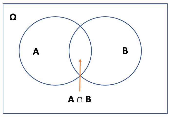
Fig 1: Conditional Probability
A simpler way of understanding conditional probability is the following: If event $B$ has definitely happened, how likely is it for event $A$ to also happen? This is answered by the fraction of times $A$ happens when $B$ happens.
Chain Rule
Chain rule of probabilities is used for Markov Models. According to chain rule, if we have 2 events $A$ and $B$, the probability of $A \cap B$ can be written as below:
\[P(A \cap B) = P(A|B) P(B)\]When events A and B occur together they are written as $P(A \cap B)$ or $P(A B)$
For $n$ events, $A_1, A_2, \ldots, A_n$, the chain rule is:
\[P(A_1 \cap A_2 \ldots \cap A_n) = P(A_1) P(A_2|A_1) \ldots P(A_n|\cap_{i=1}^{n-1}A_i)\]Another notation is:
\[P(A_1 A_2 \ldots A_n) = P(A_1) P(A_2|A_1) \ldots P(A_n|\prod_{i=1}^{n-1}A_i)\]Applying this to NLP, we can compute the probability of the sentence “Pete is happy” by computing:
\[P(Pete, is, happy) = P(Pete) P(is| Pete) P(happy| is, Pete)\]For very long sentences, such joint probabilities are very hard to compute, e.g. the probability of the sentence “I am happy because I ate salad for lunch on Wednesday” depends on the frequency of this exact sentence in the corpus. It is quite possible that this exact sentence does not exist in our training dataset, cut the component words do exist. In which case it is helpful to make an independence assumption.
Independence of Events
Two events $A$ and $B$ are independent of each other if $P(A B) = P(A) P(B)$. That means that there is no overlap between the two events with respect to Figure 1.
When applying the independence assumption, $P(A|B) = P(A)$ because the presence of $B$ does not affect the probability of $A$ at all.
Two events $A$ and $B$ are conditionally independent given an event $C$ where $P(C) > 0$ if:
\[P(A \cap B|C) = P(A|C) P(B|C)\]Bayes Theorem
According to Bayes theorem:
\[P(B|A) = \frac{P(A|B) P(B)}{P(A)}\]The denominator is a normalizing factor, and it helps produce a probability function.
If we are simply interested in which event is most likely given A, we can ignore the normalizing constant because it is the same value for all events.
Bayes theorem is central to the noisy channel model
Random Variables
Random Variables map outcomes of random processes to numbers. Random variables are different from regular variables. Random variables can have many values, but regular variables can be solved for a small set of values. The probability $P(random|condition)$ helps with the mathematics notation of probability.
The value held by a random variable can be discrete of continuous. Discrete is separate values e.g. 1, 2, 3, where as continuous is when the random variable can held any value within an interval e.g. between 0 and 1.
Probability Mass Function
Probability Mass Function (or PMF) of a discrete random variable $X$ provides the probabilities $P(X=x)$ for all the possible values of $x$.
Expectation
Expectation tells us what is the most likely outcome to expect. Expectation is the mean or average of the random variable:
\[E(X) = \sum_{x}xP(x)\]Calculating Expectation is central to Information Theory.
Variance
The variance of a random variable is a measure of whether the values of the random variable tend to be consistent over trials or to vary a lot. Variance is represented as $\sigma^2$
\[\begin{eqnarray} var(X) &=& E((X-E(X))^2 \nonumber\\ &=& E(X^2)-E^2(X)) \end{eqnarray}\]Standard Deviation
Standard Deviation is the square root of variance. It is represented as $\sigma$.
Joint Probability Mass Function
The joint probability of two events $x$ and $y$ is represented as:
\[P(x,y) = P(X=y, Y=y)\]Marginal Distribution
Marginal PMFs total up the probability masses for the values of each variable separately.
\[P_X(x) = \sum_y P(x,y)\] \[P_Y(y) = \sum_x P(x,y)\]Relative Frequency
The proportion of times a certain outcome occurs is called the relative frequency of the outcome.
$P$ - probability function
$p$ - probability mass function
We take a parametric approach to estimate the probability function in language.
Non-parametric approaches are used in classification, or when the underlying distribution of the data is unknown.
Distributions
The types of functions for probability mass functions are called distributions
- Discrete Distributions: Binomial discrete distributions are a series of trails with 2 outcomes only.
- Multi-nominal Distribution: A special case of binomial distribution is Multi-nominal Distribution where each trial has more than 2 basic outcomes
- Bernoulli distribution: A special case of discrete distributions where there is only one trial.
- Continuous distributions Continuous distributions are also known as Normal distributions
Continuous distribution
A continuous distribution is also known as a Normal Distribution or a Bell Curve. We also refer to them as Gaussians (often used in clustering). A Gaussian is represented as:
\[n(x; \mu, \sigma) = \frac{1}{\sigma \sqrt{2\pi}} e^{\frac{-(x-\mu)}{2\sigma^2}}\]Where $\sigma$ is the standard deviation and $\mu$ is the mean.
It is also the probability density of observing a single data point $x$, that is generated from a gaussian distribution.
Maximum Likelihood Estimate
Maximum Likelihood Estimate or MLE helps us identify which values of $\mu$ and $\sigma$ should we use that produce a curve that explains or covers all the data points. It is the way to determine the most likely outcome to a set of trials.
Bayesian Updating
The process of using prior to get posterior, posterior becomes the new prior, as new data comes.
\[P(\Theta|data) = P(data|\Theta) \text{ } P(\Theta)\]Here $\Theta$ is what we are interested in and what we are trying to estimate. It represented the set of parameters. If we are trying to estimate the parameters of a gaussian distribution then $\Theta$ represents both the mean $\mu$ and the standard deviation $\sigma$ and $\Theta = \{\mu, \sigma\}$
Here $P(\Theta|data)$ is the posterior and $P(\Theta)$ is the prior.
Prior belief is computed as the following:
\[P(s|\mu_m) = m^i (1-m)^j\]Here:
- $i$ = outcome of 1 counts
- $j$ = outcome of 2 counts
- $\mu_m$ is the model that asserts the outcome
- $s$ is a sequence of observations
Likelihood Ratio
Ratio computed between 2 models to see which of them is more likely to occur.
People often take log likelihood ratio and see it the result is $>$ 1 or $<$ 1
The ratio to determine which theory is most likely to occur given a sequence of events $s$.
Let $v$ be the first theory and $\mu$ be the seond theory.
\[\frac{P(\mu|s)}{P(v|s)} = \frac{P(s|\mu) P(\mu)}{P(s|v)P(v)}\]If the ratio is $>1$ we prefer theory $\mu$ (the numerator). If the ratio is $<1$ we prefer theory $v$ (the denominator).
Derivation
Derivation is the process of finding the maxima and minima of functions.
Computing the partial derivative WRT $\mu$ and then setting the equation to $0$ gives us the MLE fo $\mu$
Bayes Optimal Decision
When we pick the best decision theory out of all the available theories that could explain the data, we make the Bayes Optimal Decision.